Tips to ace your Hadamard test

In my previous medium article, we saw how the SWAP test works and illustrated some fundamentals of quantum mechanics. Typically, such test requires two quantum states (represented via circuit registers) and an ancillary qubit, whose expectation value on the z-axis (or computational basis, |0⟩ and |1⟩) yields the probability of measuring a quantum system |ψ⟩ in a specific state |φ⟩. I will display it again to refresh your memory, here is how it looks:

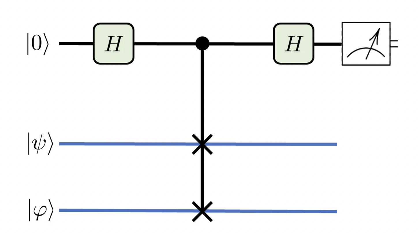
In the end, the measurements provide you an estimate of |<φ|ψ>|², that is, the probability of measuring (a system originally prepared in state) |φ⟩ in state |ψ⟩, or vice-versa. I suppose you know that, in mathematical terms, the |X|² operation gives you the absolute squared value of X — X being generally a complex number. Note that X, in our case, equals <φ|ψ>, which is the overlapbetween states |ψ⟩ and |φ⟩. Why is it useful? I can think of at least one important application of quantum state overlaps: you probably heard of orbital hybridization in your chemistry lessons, right?

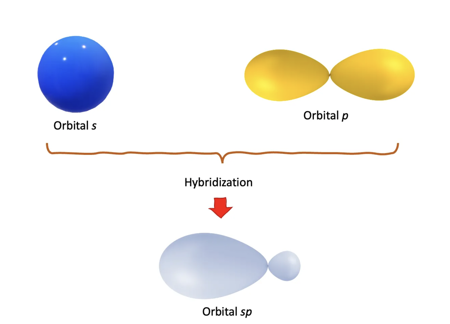
Atomic or molecular orbitals are the regions where a roaming electron is most likely to be (around the atomic nucleus or nuclei in a molecule, of course). They may differ in shape, corresponding to different energy levels or angular momenta. In the simplest cases (e.g., the hydrogen atom), these orbitals are orthogonal, meaning they do not mix, but that is not the case for composite systems, such as in molecules. In those cases, the orbitals mix and generate different geometries, so that they are no longer orthogonal. In this scenario, the overlap <φ|ψ> would measure how mixed the states have become. For example, in a methane molecule, the hybrid sp state is composed of the spherically symmetrical orbital s and the twisted balloon-like p orbitals.

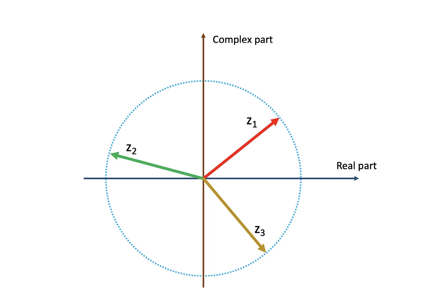
But I digress. The point is that the overlap <φ|ψ> contains more information than the probability |<φ|ψ>|², that is, you can get the probability from the overlap, but not the other way around. The reason is simple to picture if you restrict the overlap <φ|ψ> to real numbers, because the absolute value erases the original sign of <φ|ψ>. In the general case of a complex number, it erases the complex phase. For example, in the figure below, all complex numbers in the plane have the same “norm”, or absolute value, although they are all distinct from one another with respect to their complex phase.

You might wonder if complex numbers are really necessary in quantum mechanics; if that is the case, you might be surprised that there is strong experimental evidence for that. A recent article shows a setup of three observers, Alice, Bob and Charlie, who share three qubits. The authors develop a procedure of entanglement operations and measurements, from which a score is calculated. It turns out the quantum mechanics with complex numbers has a higher score than its counterpart with real numbers only. But enough meandering! let us go back to the main subject.

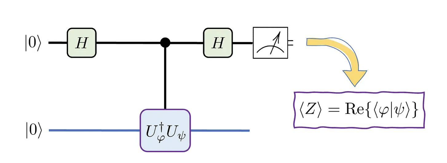
The loss of information in the SWAP test is circumvented if we use instead the Hadamard test, a depiction of which is shown below. Let us go over the most striking differences first.

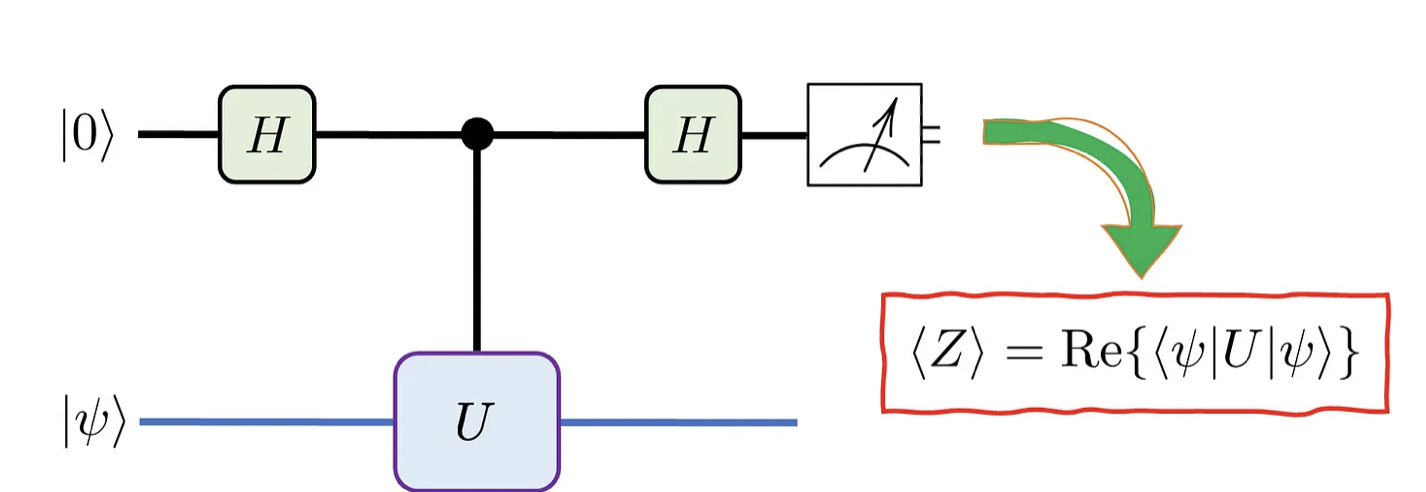
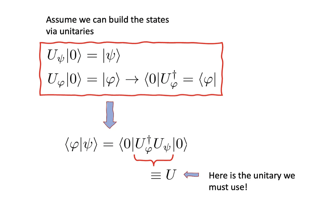
Well, first of all, you only have a single state |ψ⟩ and a controlled (general) unitary U instead of a SWAP gate. It sure looks very different from the SWAP test, but it is just in appearance, I promise you. If you want to get the (real component of the) overlap <φ|ψ>, the trick is choosing the good unitary. For that, we suppose we can create the states |ψ⟩ and |φ⟩ out of the state |0⟩. The starting point is <Z> = Re{<0|U|0>} and we will try to choose U so that <Z> = Re{<φ|ψ>}. The procedure is shown next.

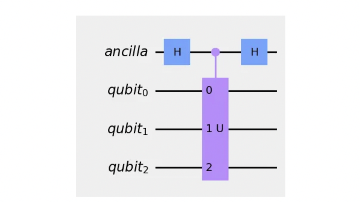
Once the unitary is built, we can use it in the Hadamard test as displayed below. Observe how it provides the real part of the overlap.

Excellent! We can obtain the real part of the overlap of two quantum states. However, we are still missing the complex part of it. Luckily, evaluating that demands only a slight change in the original Hadamard test shown above. Here is how it looks in case you want to evaluate the complex part of <φ|ψ>:

Once the Hadamard gate transforms the base states |0⟩ and |1⟩ into uniform (and mutually orthogonal) superpositions of those, the operator S† (read S-dagger) gives an additional complex phase to the |1⟩ component. Below you see its matrix representation and effect on the basis states.

As before, by keeping track of the ancilla’s measurement results, we can estimate <Z> by taking averages. We use the following procedure:

1. Count all ancilla measurements corresponding to |0⟩ and call it A
2. Count all ancilla measurements corresponding to |1⟩ and call it B
3. Estimate <Z> by averaging the results: <Z> = (A - B)/(Total number of measurements)

Unlike the SWAP test, I did not find many implementations of it online. But I guess you can consider yourself lucky, because I will put down some qiskit code here so you can see how the Hadamard test works.

An implementation of the Hadamard test

Below I copy the implementation steps in qiskit. Feel free to improve it yourself! The version of qiskit I am using is the following

Here are the imports we will need:

I built a function that creates a parametrized quantum circuit, which will then be used to create the states |ψ> and |φ>:

Next we build a function that will measure the ancillary qubit a 1000 times and average them as described above:

Now we can build the operator U (the composition of Uφ† Uψ shown in the circuit diagrams above):

Following that, we can assemble the circuit for the Hadamard test:

Before measurement, the circuit looks like this:

Using 10 000 shots, I repeated the test 100 times. I got estimates that were 3 to 4% off with respect to the analytical result of -0.2108. PS: This error may change between different runs, as the results are naturally random.

For the sake of transparency, this is the code for evaluating the overlap analytically:

Feel free to play with it, change the initial states, the number of shots and see what happens! You will notice that the more measurement shots, the closer the estimate will be from the exact value. You can find the code in ColibrITD’s GitHub!

A note on measurement statistics

In the Hadamard test, we need twice as many measurements to obtain information about the overlap, because we are estimating two quantities instead of one. You will agree that the more measurements we make, the closer our estimates will be from the actual value. This idea, also called the law of large numbers, is behind the famous Chebyshev inequality:

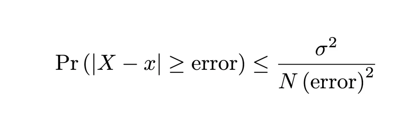
First, let us describe the elements of this formula. X is the actual value of the quantity we are estimating (the exact <Z>, in our case) , while x is our estimate after N measurements. The ‘distance’ between X and x corresponds to the error, and σ quantifies how spread the measurement statistics is. Here is how you read it: the probability that our estimate is wrong by an amount equal or larger than the error is bounded from above; this bound decreases with the inverse of the number of samples N.

A deeper analysis shows that the discrepancy (or error) (between our estimate of <Z> and its actual value) scales as ~ 1/√N, meaning that a large N provides a small error. This is the basis of many Monte Carlo algorithms, which are used to obtain estimates of quantities via random sampling.

Surprisingly, this error scaling can be improved quadratically, that is, error ~ 1/N, via the quantum amplitude estimation algorithm. It borrows ideas from Grover’s amplitude amplification and quantum phase estimation algorithms — hence the name. I intend to go over it in a future article, given its applications in quantum-enhanced Monte Carlo. A drawback of this algorithm is that it requires large scale error-corrected quantum computers, which should be available a bit farther down the road. When that happens, ColibrITD will be ready to take full advantage of them.

At ColibrITD our goal is bringing Quantum Computing for All. We use the available universal quantum computers to obtain the most quantum advantage for our customers’ use cases.