STAR WARS: IBM, AMAZON, and ATOS for Hybrid Quantum Algorithms: Fighting for Solving Differential Equations

Gozde

October 25, 2021

•

19 minutes

Introduction

Nowadays, there is a big competition in the quantum computation area since quantum computation is blooming. In the beginning, everything was simpler than today. People were just trying to build their own hardware, and some of them were building a few well-known famous algorithms (like Shor, Grover) on their hardware. What I mean is that the race included one –two hardware examples and 3–4 software tools and that was all. But currently, the race has just changed because of the potential of the hybrid algorithms and the NISQ (Noisy Intermediate Scale Quantum Era) platform. This caused a sharp increase in hardware options and software tools… The exciting point is that, while the number of tools is increasing that much sharper, a new necessity has occurred. It is quantum computation consulting. Not every company needs to build quantum computers, nor every person has to learn quantum computation, but they may need to take advantage of quantum. In this cohort, we are here. Our aim at ColibrITD is to democratize quantum computing for everyone who needs a quantum advantage. We, ColibrITD, are building a framework that includes several modules for many areas like chemistry, finance, material deformations, and security. In this tutorial, I will summarize one of our modules —VQA — for solving differential equations and we will implement it in the different hardware available — well, actually, different local simulators — The detailed explanation of it and its implementation on real quantum computer part will come with the scientific article which is on the preparation now. Stay tuned 😉

Our module: Solving differential equations (linear and non-linear set of equations and/or single equation)

Differential equations are omnipresent in science, from tracking motion in mechanics and exploring reactions in chemistry, to finding novel enhanced materials. Although there are some classical solvers for differential equations, quantum computing has the potential to accelerate computations and improve accuracy over wider domains. In this tutorial, we implement some modules of our framework to differential equations use case using local simulators of three different stars of quantum computing companies, and we will compare the results.

Image 2: Solving Differential Equations on Different Quantum Platform by Our Framework

In our framework, we have a quantum feature map and VQA modules. The
VQA module has:

A cost function library with different cost functions;
An ansatz library with Hardware Efficient Ansatz, quantum alternating operator ansatz; unitary coupled clustered ansatz, and quantum optimal control ansatz;
A classical optimization submodule with different classical optimization functions such
as ADAM, nADAM, and BFGS.

In our approach, we use a quantum feature map module, a VQA module with hardware-efficient circuits (from ansatz class of VQA module), and an original optimization method (from classical optimization class of VQA module). In practical terms, the optimization method teaches the variational quantum circuit to mimic the dynamics described in the differential equation. It is a highly effective method provided the classical optimization can be done efficiently.

Our method is based on a hybrid quantum-classical algorithm that uses quantum feature maps and a variational quantum algorithm to circumvent the inherent numerical errors of traditional finite difference methods (FDMs) Because FDMs approximate derivatives via differences between points in a discretized domain, numerical errors occur naturally. These errors propagate and, due to the nonlinearity of the PDEs, severely limit the range of validity of the solutions. Weather forecasts, for instance, illustrate how the actual solution might deviate from the prediction given enough time. This method avoids these issues by embedding the functions’ position-dependence via quantum feature map encoding, and by allowing the function’s values to be read as expectation values. Furthermore, our framework uses shallow quantum circuits, a variational quantum Algorithm (VQA) module, and a classical optimization module, so it is deployable in the currently available noisy intermediate-scale quantum (NISQ) devices.

I will explain to you the implementation of our approach on different quantum simulators. But first, I want to give you some details of the simulators that we used to implement our approach. Let us start with Amazon-Braket.

AMAZON Braket

It is the youngest one, but we should show respect for the passion of the young spirits. It introduced Quantum World at the end of 2019, the beginning of 2020. In August 2020, we had AWS Braket. AWS showed its ambitions with this amazing paper: https://arxiv.org/pdf/2012.04108.pdf. The paper came from Caltech but the people who authored the paper are now associated with Amazon Web Services to build them a quantum computer, so it is a serious business. AWS currently does not have a quantum computer, but it provides us access not only to gate-based quantum computing hardware but also to quantum annealing quantum hardware. If you have a research proposal, or if you are a researcher, you can apply for credits, otherwise, you must pay to use to access these quantum computers or high-performance simulators. Apart from them, we can use Amazon Braket python SDK with the local simulator for free. The documentation is very clear and comes with many examples. Here is the schematic of Amazon Braket:

In Amazon Braket, the atomic request to a device is a task. For gate-based QC devices, this includes the quantum circuit (including the measurement instructions and number of shots), and other request metadata. For annealing devices, it includes the problem definition, the number of shots, and other optional parameters.[1]

Amazon Braket provides us managed Jupyter notebooks (1) that come pre-installed with the Amazon Braket SDK so that you do not have to install SDK in your local laptop and you do not have to suffer from installation. You can build your quantum circuits directly in the SDK or, for annealing devices, define the annealing problem and parameters. The Amazon Braket SDK also provides a plugin for D-Wave’s Ocean tool suite, so you can natively program the D-Wave device. After your task is defined, you can choose a device to execute it on, and submit it to the Amazon Braket API (2). Depending on the device you chose, the task is queued until the device becomes available, and then it is sent to the QPU or simulator for execution (3). Amazon Braket gives you access to 3 different types of QPUs (D-Wave, IonQ, Rigetti) and managed simulators, such as SV1. To learn more, see Amazon Braket supported devices.

After your task is processed, Amazon Braket returns the results to an Amazon S3 bucket, where the data is stored in your AWS account (4). At the same time, the SDK polls for the results in the background and loads them into the Jupyter notebook at task completion. You can also view and manage your tasks on the Tasks page in the Amazon Braket console, or by using the GetQuantumTask operation of the Amazon Braket API. [2]

‍

In this tutorial, we compare the simulators of quantum computing masters. So now let us look at the simulators of AWS Braket. There are four different simulators that are given us here.

One of them is the local simulator in the Amazon Braket SDK that is provided at no cost, and we can it run on our laptop, or within an Amazon, Braket managed notebook. The local simulator is well suited for running small and medium-scale simulations up to 25 qubits without noise or up to 12 qubits with noise, depending on your hardware. You can use the local simulator for rapid prototyping, debugging or testing, before running your circuit on high-performance managed simulators and quantum computers.[3]

The second one is the StateVector simulator. It is a fully managed state vector simulator for quantum circuits. A state vector simulator takes the full wave function of the quantum state and applies the operations of the circuit to calculate the result. You can use SV1 after you have designed your quantum algorithm in the Amazon Braket SDK with the local simulator, and then test your algorithm at scale using the parallel processing of SV1 to run batches of simulations. SV1 supports simulations up to 34 qubits.[3]

The third one is the DensityMatrix simulator. It is a fully managed simulator that uses density matrix calculations to simulate the effects of noise on quantum circuits. With DM1, you can specify realistic error models for your circuits and study the impact of noise on your algorithms. DM1 supports the simulation of circuits up to 17 qubits. [3]

The last one is the TensorNetwork simulator. It is a fully managed tensor network simulator used for structured quantum circuits. A tensor network simulator encodes quantum circuits into a structured graph to find the best way to compute the outcome of the circuit. You can use TN1 to simulate certain types of quantum circuits up to 50 qubits in size. [3]

As I mentioned above, we will use the local simulator for this tutorial since it is available for everyone at no cost.

IBM

As we know, IBM is the oldest one in this kingdom. It is old but gold too 😊. It provides us access to its own quantum computer. It tends to update/refresh itself every day. There are many quantum computers that are already retired: https://quantum-computing.ibm.com/lab/docs/iql/manage/systems/retired-systems

Its technology is based on superconducting qubits as it is written on the webpage:

“IBM Quantum systems, based on IBM Quantum System One, are built using world-leading quantum processors, cryogenic components, control electronics, and classical computing technology.”

These systems are denoted by names that start with ibmq_*. All systems return a configuration file containing all the information needed for executing quantum circuits on the systems. Additionally, quantum systems return properties information that details the characteristics of the system qubits, as well as the gates acting on these qubits. This includes noise information obtained from system calibration scripts. [4]. The 5-qubit quantum computer is free. But the higher qubit and the more professional one, you can either pay or you can access as a researcher. Also, you can use qiskit with a local simulator at no cost. So now let us look at IBM’s simulator with details. We have five different simulators. The following simulation methods are currently available and support a maximum of 300 circuits and 8192 shots per job.[5]

Statevector Simulator is the default choice simulator as it is a general-purpose solution method.

Type: Schrödinger wave function

Name: simulator_statevector

Simulates a quantum circuit by computing the wavefunction of the qubit’s statevector as gates and instructions are applied. Supports general noise modeling.

Qubits: 32
Noise modeling: Yes

Supported gates/instructions

[‘u1’, ‘u2’, ‘u3’, ‘u’, ‘p’, ‘r’, ‘rx’, ‘ry’, ‘rz’, ‘id’,’x’, ‘y’, ‘z’, ‘h’, ‘s’, ‘sdg’, ‘sx’, ‘t’, ‘tdg’, ‘swap’,’cx’, ‘cy’, ‘cz’, ‘csx’, ‘cp’, ‘cu1’, ‘cu2’, ‘cu3’, ‘rxx’,’ryy’, ‘rzz’, ‘rzx’, ‘ccx’, ‘cswap’, ‘mcx’, ‘mcy’, ‘mcz’,’mcsx’, ‘mcp’, ‘mcu1’, ‘mcu2’, ‘mcu3’, ‘mcrx’, ‘mcry’,’mcrz’, ‘mcr’, ‘mcswap’, ‘unitary’, ‘diagonal’,’multiplexer’, ‘initialize’, ‘kraus’, ‘roerror’, ‘delay’]

Stabilizer Simulator

Type: Clifford

Name: simulator_stabilizer

An efficient simulator of Clifford circuits. Can simulate noisy evolution if the noise operators are also Clifford gates.

Qubits: 5000
Noise modeling: Yes (Clifford only)

Supported gates/instructions

[‘cx’, ‘cy’, ‘cz’, ‘id’, ‘x’, ‘y’, ‘z’, ‘h’,’s’, ‘sdg’, ‘sx’, ‘swap’, ‘delay’, ‘roerror’]

Extended stabilizer

Type: Extended Clifford (e.g., Clifford+T)

Name: simulator_extended_stabilizer

Approximates the action of a quantum circuit using a ranked-stabilizer decomposition. The number of non-Clifford gates determines the number of stabilizer terms.

Qubits: 63
Noise modeling: No

Supported gates/instructions

[‘u0’, ‘u1’, ‘cx’, ‘cz’, ‘id’, ‘x’, ‘y’, ‘z’, ‘h’,’t’, ‘tdg’, ‘s’, ‘sdg’, ‘sx’, ‘swap’, ‘p’, ‘ccx’, ‘ccz’,’delay’, ‘roerror’]

MPS

Type: Matrix Product State

Name: simulator_mps

A tensor-network simulator that uses a Matrix Product State (MPS) representation for the state that is often more efficient for states with weak entanglement.

Qubits: 100
Noise modeling: No

Supported gates/instructions

[‘unitary’, ‘t’, ‘tdg’, ‘id’, ‘cp’, ‘u1’, ‘u2’, ‘u3’, ‘u’,’cx’, ‘cz’, ‘x’, ‘y’, ‘z’, ‘h’, ‘s’, ‘sdg’, ‘sx’, ‘swap’,’p’, ‘ccx’, ‘delay’, ‘roerror’]

QASM

Type: General, context-aware

Name: ibmq_qasm_simulator

A general-purpose simulator for simulating quantum circuits both ideally and subject to noise modeling. The simulation method is automatically selected based on the input circuits and parameters.

Qubits: 32
Noise modeling: Yes

Supported gates/instructions

Here, we chose the QASM simulator since it has many operations in its. Once again, we will access the state vector and the amplitudes by a clever calculation. You will find the details of our method in the following chapters.

ATOS

Atos is a French company that built a quantum learning machine. ATOS QLM benefits are:

Bootstrap in Quantum Computing
Easy end-user quantum programming language, a set of provided Quantum Libraries, and a Jupyter Notebook environment
Program and execute hybrid quantum-classical algorithms
Integrate with existing frameworks to leverage algorithms developed via other frameworks
Support real noise simulation models on different hardware
Simulate different technologies through its hardware agnostic environment with unprecedented performances.
Explore both digital and analog quantum computing technological approaches

ATOS QLM provides us myQLM tool which is a quantum software stack for writing, simulating, optimizing, and executing quantum programs on our laptops. Through a Python interface, it provides

powerful semantics for manipulating quantum circuits, with support for universal as well as custom gate sets, abstract parameters, advanced linking options, etc.;
a versatile execution stack for running quantum jobs, including easy handling of observables, special plugins for carrying out NISQ-oriented variational methods (such as VQE, QAOA), and easy API for writing customized plugins (e.g for compilation or error mitigation), as well as for connecting to any Quantum Processing Unit (QPU);
a seamless interface to available quantum processors and major quantum programming frameworks. [6]

ATOS QML is specialized for NISQ devices and hybrid algorithms — particularly quantum machine algorithms and variational quantum algorithms — and it simulates the algorithms efficiently as it mentioned in the following. It is also easy to install. With myQLM, we can develop quantum algorithms on our laptop, we can write our own quantum processing methods and we can collaborate with any other framework users like Qiskit, Cirq, ProjectQ.

Solving (non)/linear equations with variational quantum circuits: a comparison

Let us start to implement our method for solving (non)/linear equations with differentiable quantum circuits to these platforms and see what is happening 😊

Our method can be divided into two partially overlapped parts:

state preparation
Variational Quantum Algorithm (VQA) module.

In the first part, we encode the functions and their derivatives into quantum states. In the second, we teach a Variational Quantum Circuit (VQC) to mimic the differential equation. This teaching is no more than optimization of the VQC parameters to ensure our solution satisfies the relevant PDE, along with its boundary conditions, in a certain region. The functions are read as expectation values of observables, suitably chosen cost-functions, hence avoiding the full knowledge of the quantum state, which potentially eliminates the quantum advantage. The VQA optimizes the VQC parameters so as the solution fits the PDE and boundary conditions in the desired domain, according to previously defined error acceptance rates. Here is the schematic of VQA:

Implementation Steps

Quantum Feature Map:

The first and most basic element in our workflow is the quantum feature map, used to represent functions and their derivatives. We start by the representation of functions of two variables, for illustration purposes.

In this case, the quantum feature map is a double layer of single-qubit rotations, where the angles are nonlinear functions of x and y. There are many choices for these functions, but among the most popular are n-order Chebyshev polynomials or other complete sets of orthonormal functions. The idea is to choose functions with a high level of representability, which is the case of complete sets of functions. In our proof-of-principle, we chose the n=1 order Chebyshev encoding, which means we chose the following function phi:

In this module, we used Chebychev Encoding phi(x).

Modeling the Differential Equation:

The differential equations are modeled as a functional equation whose fit is measured by a loss function. The evaluation of the PDE is done classically using its quantum-evaluated elements, i.e., its functions and derivatives. Typically, the PDEs can be written as:

For random VQC parameters, this function should not yield zero as the parameters are not optimized for the PDE. The goal of the optimization loop is to teach the VQC how to mimic the PDE dynamics. Before, however, we go over two possible choices of cost functions.

Cost Function

The cost function is fundamental in evaluating functions and derivatives and should be a function that is efficiently evaluated by a quantum computer. Observe, however, that the possible outcomes of this function should at least span the range of values acceptable for the function. For example, say we dispose of 6 qubits. Choosing the cost function as the total magnetization limits us to describe functions that range from N=-6 to N=6

Because each qubit will return either Zi=-1 or Zi=1. This is sufficient for, say, expressing 6.cos(x.y), but not for tan(x.y). A more versatile choice of the cost function is

where the ci are also subject to optimization and the cost functions Ci are efficiently evaluated by a quantum computer. This second choice is desirable should the function span larger values. Still, other cost functions can be used, such as the Ising model or nearest neighbor Hamiltonians.

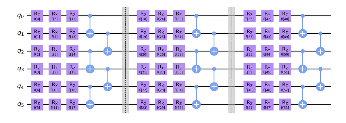
Ansatz

The Ansatz is the term referring to the parametrized quantum circuit used in the Variational Quantum Circuit. It is defined as a succession of gates, controlled or not, depending on parameters. These gates can sometimes be regrouped into layers, making it the quantum analog of the classical neural network architecture. By tuning and adjusting these parameters, the goal is to build a quantum circuit that can generate specific states at the output, useful for approaching other circuits, computing cost functions, or retrieving quantum states that contain solutions to the problem.

The rotations, all generic manipulations of single qubits, and the controlled gate are responsible for the entanglement between the particles, allowing the circuit to be more expressible and to span a large class of quantum states.

A good choice of variational ansatz is also important in loss-function-convergence success and speed. In fact, for tackling the problem in the challenge, we choose to use Hardware Efficient Ansatz since it keeps the circuit depth short, minimizes the noise, and keeps the number of gates low. For higher depths, the number of tunable parameters increases, and one may find barren plateaus, which must be dealt with with smart classical optimization approaches. Still, Hardware efficient ansatz is fundamental for every type of hardware topology. In fact, current noisy quantum computers (such as AMAZON or IBM) benefit from Hardware Efficient ansatz due to their low levels of noise.

Loss Function

The loss function, as the name suggests, tells us how much information our optimization iteration misses; our goal of course is minimizing it. The solution of a PDE must respect both the PDE functional and the boundary conditions. These two criteria can be allocated in the loss function as

The first term evaluates the fit to the differential equation, while the second account for the fit at the boundaries or initial conditions. In both terms, we use the mean squared error of N samples as a loss function. For instance, the PDE-part of the loss function should look like this:

where the function is evaluated at different points of the domain; observe we wrote the value zero explicitly to emphasize this should be the target-value.

Classical Optimization:

In order to find the solution to the problem, one must find the best parameters that define the Ansatz. This is done through the optimization of an objective function. This objective function is the loss function defined previously, which links the value of the parameters directly with the problem to be solved.
The goal of the classical optimization step is thus to leverage classical optimization algorithms to minimize the loss function in order to find the best parameters of the ansatz needed for solving differential equations.

In the context of Variational Quantum Circuits, gradient-based optimization methods (such as ADAM) are the most used in the literature. They provide fast convergence when the objective function is convex, when the derivative of the objective function is available and when they are combined with an accurate initialization of the parameters.

In our approach, the loss function is not convex, and its gradient is not easily expressible. Besides, we plan to work on the initialization of the parameters, but the strategy is not yet ready. Therefore, if we use the gradient-based optimization method, we will most of the time converge to one of the local minima instead of the optimal solution that permits us to solve the problem. Because of this problem, we implemented our own original algorithm which will be defined in our incoming paper.

Implementation of the Method and Comparison of the Platforms with a Specific Differential Equation

I will now explain some parts of the code for these three different structures: As in ref. [9] we take a simple differential equation just to show how to implement our VQA module and the differential equations method can be implemented:

Subject to the initial condition y(0)=1. This ODE admits the following analytical solution

which represents a transient oscillation pattern.

We chose the magnetization cost function for our problem. Implementation of it is independent from the platforms since it is a function without any quantum gate/structures
The other crucial step is to quantum feature map. You can use any complete basis of polynomials. This part can be implemented as a simple function that has no differences between different platforms since it is a mathematical function.
We need to find its derivative: d(phi)/dx: This function is also a simple mathematical function so nothing will change for the platforms.
Single Variable QFM:

Here, although we have different syntax for the platforms, the structure is of course the same:

For AWS-Braket:

For IBM Qiskit

For ATOS-myQLM

For AWS-Braket, we simply create a circuit from a Circuit object without specializing the size of the circuit.

For IBM Qiskit, we create a Circuit instance with QuantumCircuit object, but we need to specialize in the dimension of the circuit. Also, IBM Qiskit provides us with a barrier structure which is very useful and important for the order processing of the circuit.

For ATOS myQLM, we create the Circuit from the Program, also we need to create our qubit from qalloc structure.

4. QFM for derivatives

To calculate it, we have four different functions

a. State base derivative:

It returns a circuit with the j-th qubit rotated by an additional angle pi/2

:param x: real between ]0,1[

:param n: order of the encoding

:param N: integer, number of qubits

:param sign: sign of the C-operator, enter: +1 or -1

:param j: CIRCUIT with the j-th qbit rotated by an extra angle (sign)np.pi/2, with j in range(0,N)

b. Ansatz which was explained in the above with detail and I put the schematic of our ansatz for this method instead of putting the code. For building ansatz, we directly used our ansatz class of our VQA module. There is no difference between different platforms apart from the ones defined in the QFM above

c. We also need to following function which is necessary for the derivatives Here I put half part of the code just to explain the differences between platforms

For AWS-Braket

For IBM Qiskit

‍For ATOS myQLM

Here, as can be seen clearly:

For AWS-Braket we directly call the local simulator, we do not need to create a job and we can write everything in one line for getting probabilities.
For IBM Qiskit, (with the QASM simulator) we need to create a job after calling the simulator. Then for accessing probabilities, we first access the amplitudes from the statevector of the state and then we multiply the amplitudes by square, and then finally we have the probabilities
For ATOS myQLM, we call the simulator with “get default qpu”, then we create a job and then we submit the job and after that, we can access the probabilities from the result of the sample without dealing with the amplitudes.

Here I must say that AWS-Braket is quite good in terms of accessibility and codeability.

d. Finally we sum our probabilities for each run for C+ and C- with the simulate_magnetization function.

5. Evaluation of the Cost Function

To find the evaluation of Cost function, we have 2 different functions:

a. First, we compute the expectation value of total magnetization representing the function at position x. We adapted the function to deal with floating boundary conditions. Here the differences between the platforms are the same as the differences above

b. We compute how far the loss function is from zero

6. Classical Optimization

We wrote our own Optimization method instead of using a ready library and this gives us the freedom to change/manipulate it when it is needed. A suitable optimization algorithm finds the right parameters and gives us perfect fitting. Now, to conclude this tutorial, we will give the same parameters for each platform, and we will see how curves are fit and how long it takes to run.

Results:

In this part, we will see the time and accuracy for each platform with the same optimization parameters:

(Please note that these parameters are not optimal. They were chosen solely for comparing platforms.)

Amazon — Braket: