Are you terrified of being asked about the fundamentals of quantum mechanics while making small talk in the elevator? If yes, this article is made for you. Well, at least the first part of it.
As you should expect, this article is about the SWAP test, a procedure to evaluate probabilities in quantum mechanics. But because this test involves many core aspects of the theory, I will take advantage of it to highlight some of them. Let us start by illustrating some similarities and differences between classical and quantum mechanics.
Classical versus Quantum mechanics
You see both are “mechanics”, right? This means both are theories that describe how stuff responds to stimuli; how they evolve with time, given an initial configuration. This overall behavior of a system is often called dynamics, in Physics terms. But that is as far as the similarities go. That was quick! Now let us go over the very interesting differences.
In tangible terms, you can develop a zillion physical theories, but if any of them is to be considered “valid” at a given moment, they must agree with observations and experiments, and make predictions. This is particularly tricky with quantum and classical mechanics, because it is often thought they are applicable in mutually exclusive realms: the microscopic and macroscopic. But this is an illusion (have a look at my colleague Marta Reina’s Medium article).
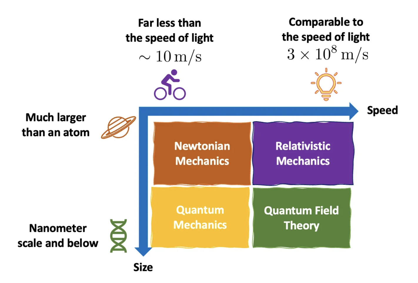
While classical mechanics (Newton’s laws and classical Electrodynamics) fails in describing the behavior of atomic systems (in the scales of nanometers and below), quantum mechanics not only describes such systems, but it also applies to macroscopic objects. In fact, experiments have pushed the observation of quantum phenomena to the scale of micrometers, a remarkable feat that was Physics World’s 2021 breakthrough of the year [1]. Accordingly, you can even make the case Newton’s laws are wrong, which does not make them useless, as using quantum mechanics to describe macroscopic phenomena is like killing a [insert a delicate living target here] with a [insert a powerful weapon or heavy tool here].
Ultimately, classical mechanics fails because it does not capture the dual wave-particle behavior, graininess, and probabilistic nature of quantum systems. I will follow these three characteristics because in the end they will help us understand how the SWAP test works.
Wave-particle duality
This characteristic is very conspicuous in light, and Young’s double slit experiment is a great way to illustrate it. The setup is very simple: an opaque wall with 2 slit openings is set between a light source and another opaque wall without slits, which we call screen.
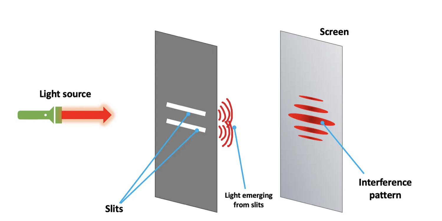
As we turn on the light source, a pattern of fringes appears on the screen: a series of illuminated strips, the central one the brightest if our setup is symmetrical. This pattern is easily explained if we assume light is a wave, because waves display interference; the light (dark) fringes are regions with constructive (destructive) interference between the wavefronts that leave the two slits and recombine at the screen’s surface. Now let us try something slightly different.
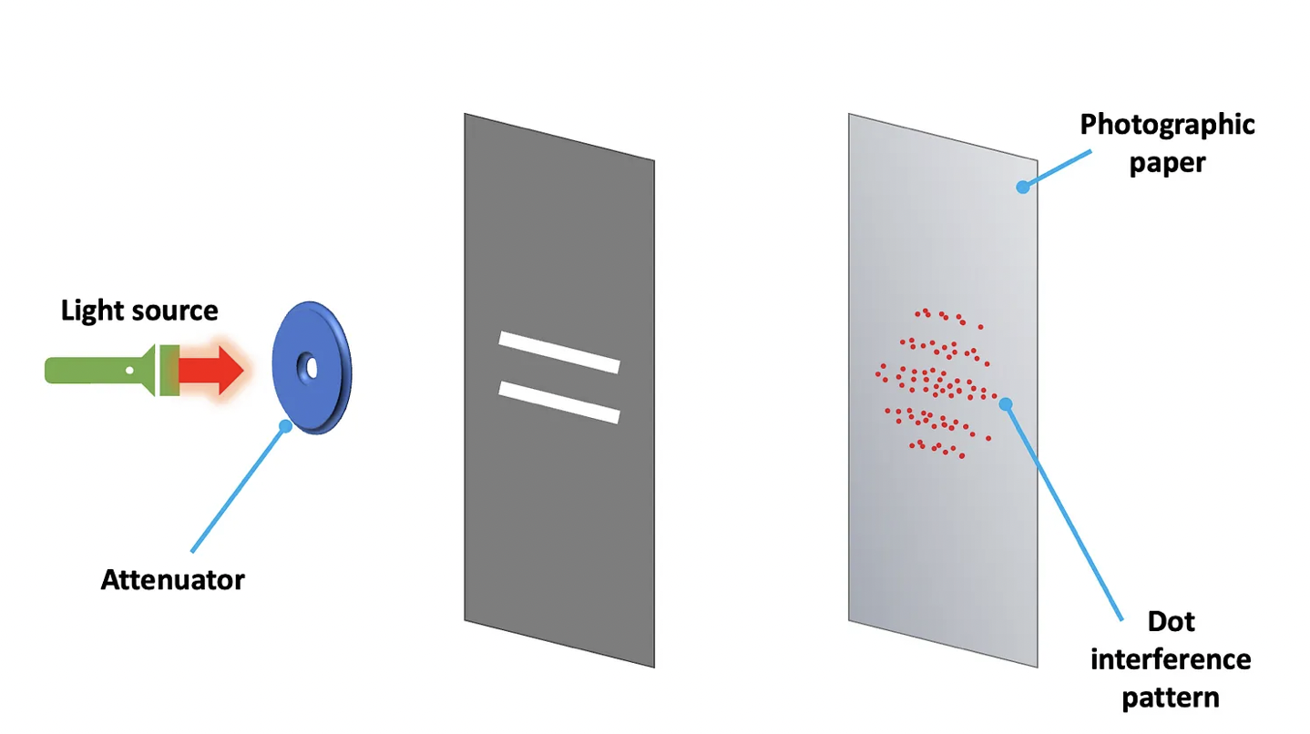
Say we now make the light very but very weak by using an attenuator between the slits and the source. Also, instead of an opaque screen, say we use photographic paper. If the light is weak enough, you will see individual points appear in the photographic paper. These are the result of individual “photons”, the quanta or particles of light. If you wait long enough, the overall distribution of points should match the one from the previous setup. Some will be tempted to say light propagates like a wave, but when it comes to its detection, it behaves like a particle. Physicists would probably like this observation. Such duality has very deep implications.
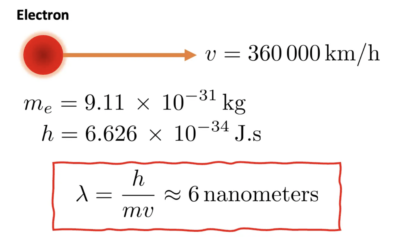
If light can display particle- and wave-like behavior, could matter do the same? The answer is yes, as formalized by the French physicist Louis de Broglie in 1924, who introduced the concept of matter waves. According to his hypothesis, a massive particle with momentum p has an associated wavelength λ of λ = h/p, where h is the Planck’s constant.
A possible interpretation is that each individual photon interferes with itself and goes through both slits at the same time, becoming then a superposition of the quantum states |upper slit⟩ + |lower slit⟩. The word “state” is used on purpose here, as quantum systems are described fully by their states. In fact, all there is to know about the quantum system in question is in its quantum state, or wave function*.
The graininess of quantum systems
For the sake of the reader’s patience, I will try to be short here. By graininess I mean that quantum states can be discrete (countable), as opposed to continuous. It just means you can often label them. Above, you saw that the photon’s state is a superposition of only two states: |upper slit⟩ and |lower slit>.
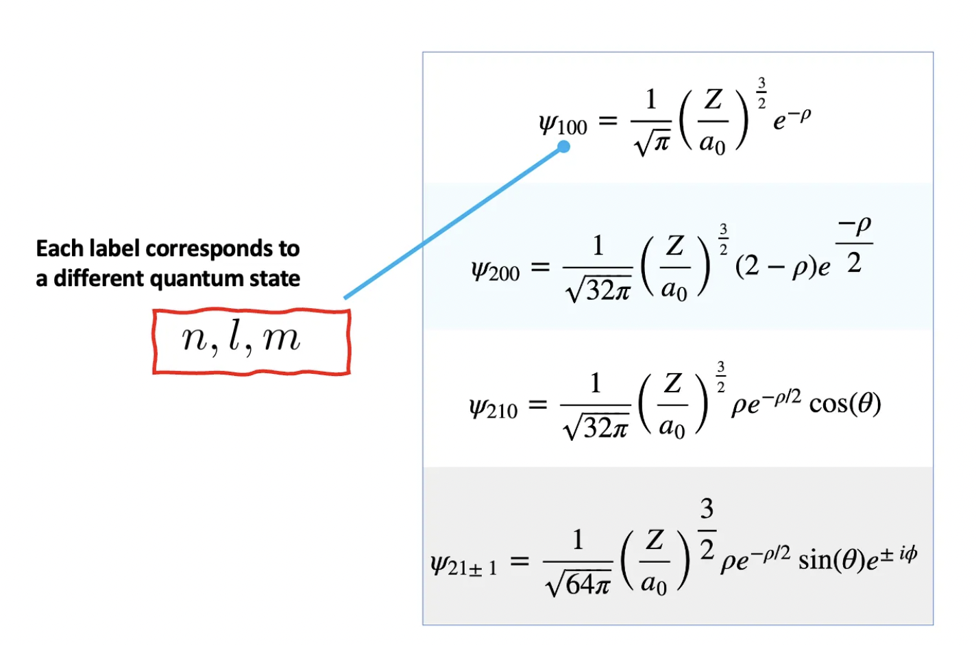
These labels should not come as a surprise. You remember the principal, secondary and magnetic quantum numbers (n, l, m) that we study in chemistry? They are labels of the wave functions that describe the electronic distribution around an atom. I’ll list some below. Labelling them is much easier than writing them in full, isn’t it?
Another example of graininess is the atomic spectrum. The word sounds ominous, but it is a very simple idea. An atom in a state with a label A can sometimes jump or transition to state B, and vice versa. Most commonly there is an energy difference between them, which means either the atom absorbs or emits that amount of energy. In practice, if you make incoherent light (like the Sun’s) go through a cloud of these, you will observe some wavelengths are missing. These very same wavelengths are the only ones displayed if the atom cloud is excited, or heated, for example. See the figures just below. You see another example of discreteness here?

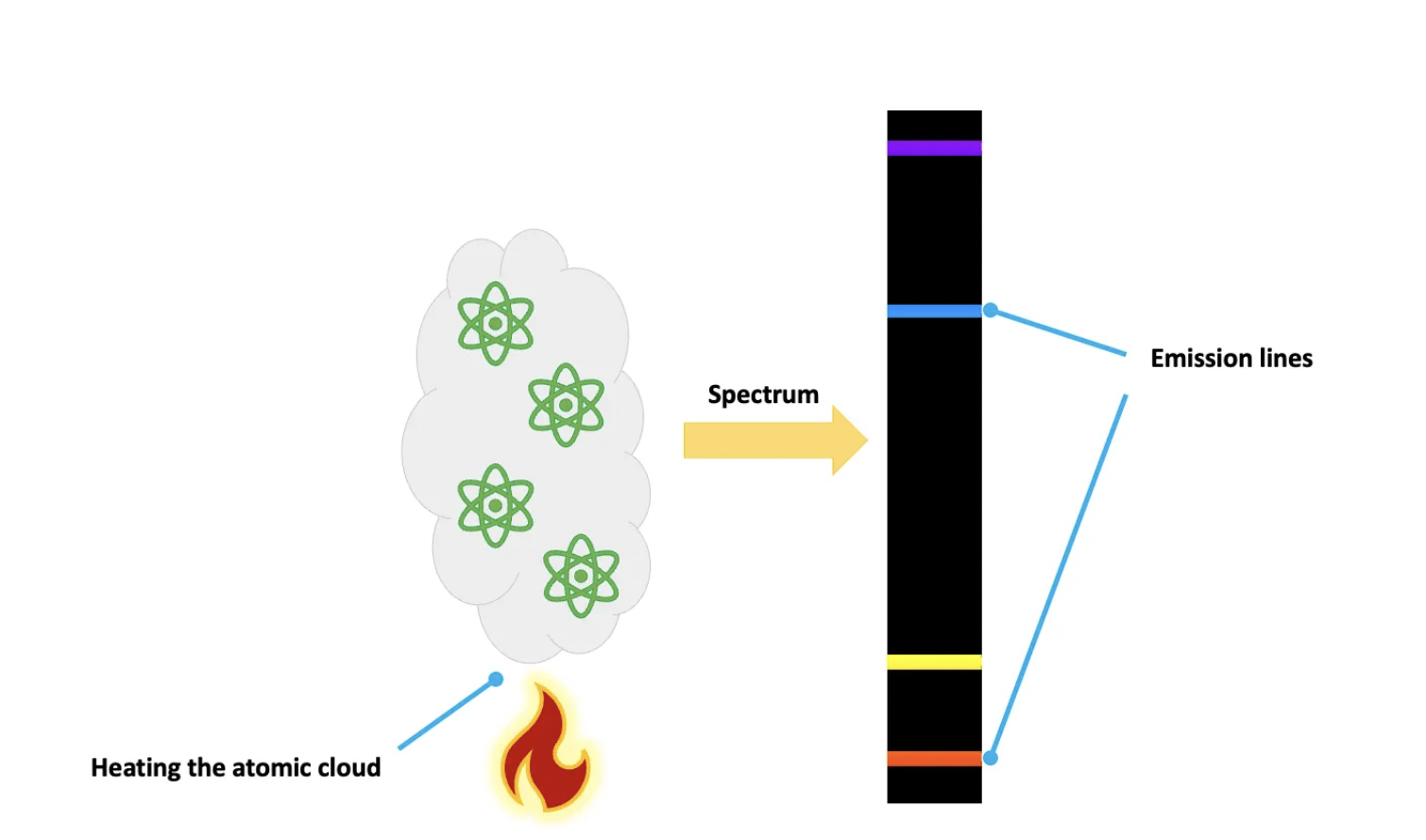
The set of wavelengths (or energies, conversely) emitted or absorbed constitute the atomic spectrum. See, for instance, the Rydberg series.
Now to the probabilistic aspect of quantum mechanics.
Probabilities and the SWAP test
This aspect is easy to picture with superposition. Consider the double-slit experiment again. In that case, after the slits, the photon’s state is a superposition of |upper slit⟩ and |lower slit⟩. You may ask yourself: “Does it really go through both slits at the same time or we simply do not know through which one it goes?” or even “What happens if I try to see through which slit the photon goes?”.
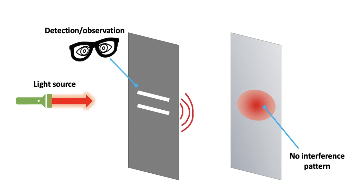
If you try it, you will get an answer: either |upper slit⟩ or |lower slit⟩, at the cost of losing the interference pattern in the screen. In that case, we say the observation (or measurement) collapsed the quantum state into one of the basis states. The wavefunction’s collapse does not happen every time an observation is done. For example, after measurement, the state may not change, so that a successive measurement does not collapse the wavefunction, as it merely stays in the same state as before.
In any case, after the measurement, the system ends up in a particular state according to certain probabilities. This process is ultimately random. In a later article I shall talk about this probabilistic facet of Nature and our idea of determinism.
To find the probability of a system to be found in a particular state we recall the 2nd postulate (this number may vary) of quantum mechanics:
Given a quantum state |ψ>, the probability of it being measured in state |φ>
is given by: |<φ|ψ>|² .
The product <φ|ψ> is called an inner product and it yields a number, generally complex, or a scalar in the proper lingo; it must satisfy certain properties — you can find them here. Because |<φ|ψ>|² is a probability, it must range between 0 and 1 (for normalized states). It is 0 for it being impossible, and 1 for it being certain |ψ⟩ will be measured in state |φ>. In case it is impossible (|<φ|ψ>|² = 0), we say |φ⟩ and |ψ⟩ are orthogonal — the states have nothing in common.
Concretely, the probabilities are obtained after averaging over many repeated measurements, because the outcome of the measurements are random, except the extreme cases just mentioned.
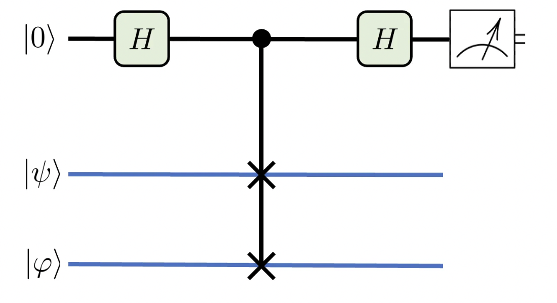
If, like myself, you ever wondered how to evaluate |<φ|ψ>|², the SWAP test does just that. It gets its name from the SWAP gate used in its circuit representation.
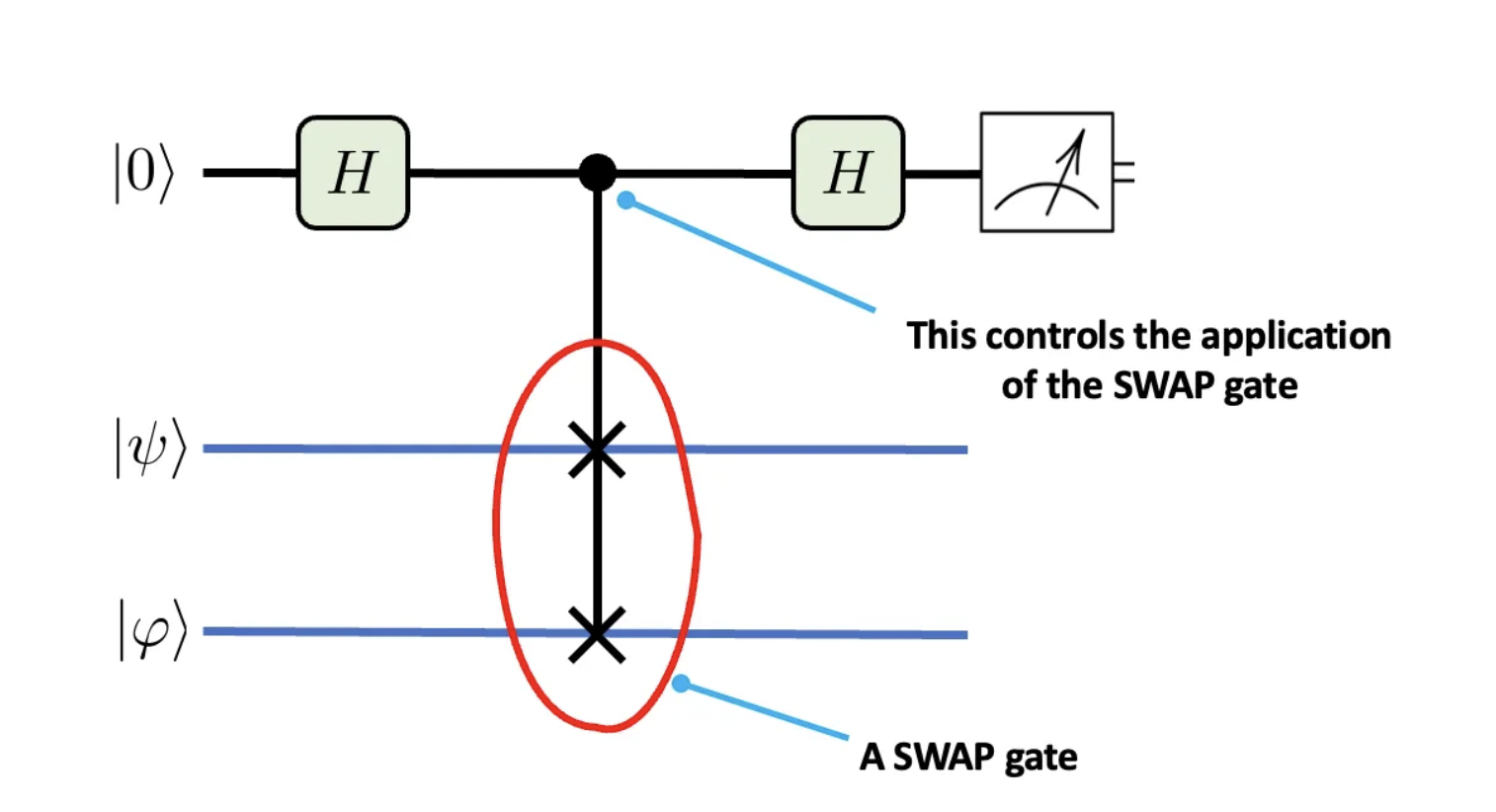
On the top is the ancillary qubit, the only one we will measure, as indicated in the rightmost operation. By using Hadamard gates and a controlled-SWAP gate, the whole system is put in a superposition of mutually exclusive states. There are some excellent online resources that go over the underlying math of this operation [2, 3]. In the end, measuring the ancillary qubit yields 0 or 1. So how do you use it to evaluate |<φ|ψ>|²? Bear with me!
Working the math out, the probability of measuring the ancillary qubit in state |0⟩ is given by:
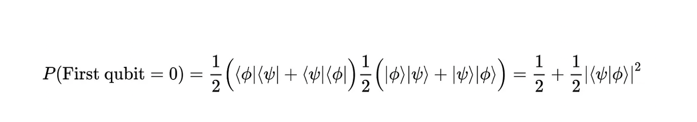
If you somehow find P, you get |<φ|ψ>|². You can do it by repeating the test many times, recording the results and then averaging them as in the following:

And voilà! You get |<φ|ψ>|² like this:
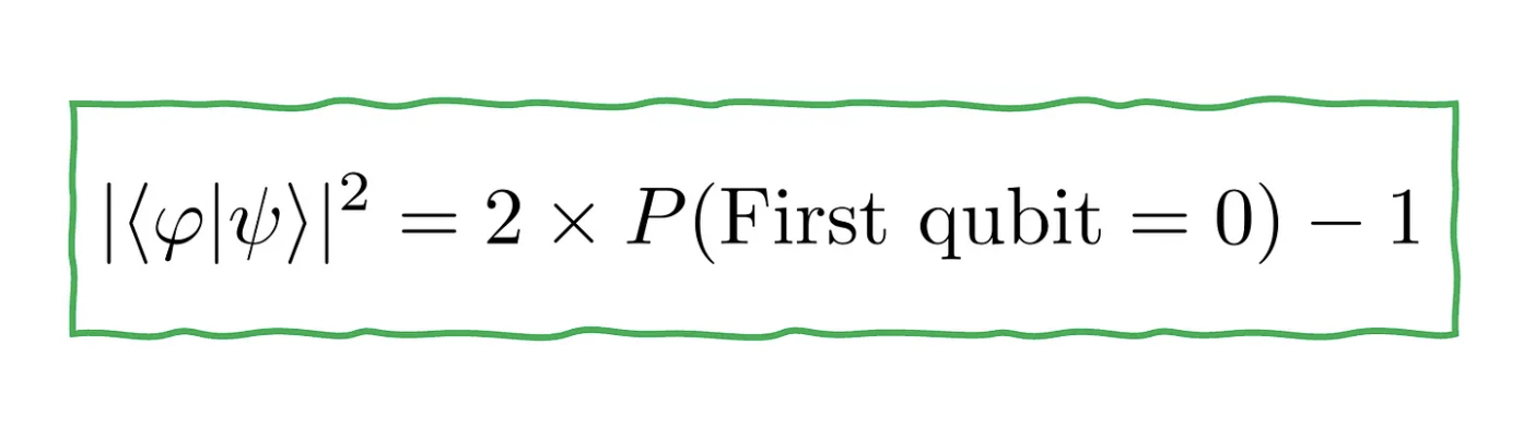
The more measurements you do, the more precise the estimation is. Observe that the probability |<φ|ψ>|² is the absolute square of <φ|ψ>, which is in general a complex number. It is called an overlap and appears very often in the study of chemical bonds, for example. To evaluate it, we need a different scheme, called a Hadamard test, which I will cover in the next article — please do not look up for spoilers.
At ColibrITD our goal is bringing Quantum Computing for All. We use the available universal quantum computers to obtain the most quantum advantage for our customers’ use cases.
References
* To be precise, they are not quite the same thing, as Sakurai’s great books tell, but I will ignore the distinction here. Here is the book info:
Modern Quantum Mechanics (2nd Edition) 2nd Edition by J. J. Sakurai, Jim J. Napolitano. Pearson, 2010.
[2] https://en.wikipedia.org/wiki/Swap_test
[3] https://quantumcomputinguk.org/tutorials/introduction-to-the-swap-test-in-qiskit-with-code
Discover the Latest Blog Posts
Experience FASTER and More Efficient Computing with Our Quantum Solution


