Getting to Know Quantum Fourier Transform

Joseph Fourier (1768 –1830) is a french mathematician and physicist. He is known for having determined, by calculus, the heat diffusion by using the decomposition of an arbitrary function thanks to his famous Fourier series.

One motivation for the Fourier Transform comes from the study of the Fourier series. In the study of the Fourier series, complicated but periodic functions are written as the sum of simple waves mathematically represented by sines and cosines. The Fourier Transform is an extension of the Fourier series that results when the period of the represented function is lengthened and allowed to approach infinity [W]. The Fourier Transform can also be adapted to a discrete version, which is named the Discrete Fourier Transform (DFT).

The Quantum Fourier Transform (QFT) is the quantum analog of the DFT and is a central tool in Quantum Computing. It is an important step in the period-finding quantum algorithm, permitting to reveal of periodic aspects encoded in a quantum state.

In this article, we present the Quantum Fourier Transform from different angles, recalling its fundamental properties and representations. Since Quantum Entanglement is the key resource in Quantum Computing, we propose to study its relation with this transformation, i.e. how QFT creates or modifies the entanglement of small quantum systems.

“Quantum Fourier Transform is an important part of many quantum algorithms, most notably Shor’s factoring algorithm and Quantum Phase Estimation”

IBM Quantum

From Classical to Quantum Fourier Transform

We recall that the DFT transforms a sequence of N complex numbers

into another sequence of N complex numbers

by the following relation [W2]:

The definition of the Quantum Fourier Transform is quite analogous to the DFT definition. In fact, we consider the computational basis {|0⟩,|1⟩,…,|N-1⟩}(in decimal notation), with N=2^n, where n is the number of qubits. The action of the QFT on one of the basis states |k⟩ is described by the following expression:

Any quantum state |ψ⟩ can be written as a linear combination of the basis states (superposition principle). Therefore, since the QFT is a linear operator, it acts on a general quantum state |ψ⟩ as follows:

, with each amplitude itself defined as:

Matrix representation of the QFT

By using the expression above, one can describe how the QFT transforms each vector of the computational basis. We can thus construct the associated N x N matrix as follows:

Circuit representation of the QFT

The Quantum Fourier Transform can also be decomposed into several basic quantum gates, acting on one or two qubits. This permits us to easily represent graphically the operator as a quantum circuit, which is always relevant in the context of quantum algorithms study and development (which is my main activity at ColibrITD).

Indeed, the QFT can be defined as a combination and succession of three different gates: the Hadamard gate, the SWAP gate, and the controlled-Rk (defined below).

The complete circuit of the QFT is represented below, and the last gate is SWAPn, the n-qubit gate consisting in swapping the first qubit with the last, the second with the (n-1)-th qubit, and so on.

One of the reasons why the QFT is so important in quantum computing (especially in quantum algorithms) is the fact that the complexity of the QFT is quadratic in the number of quantum gates involved in its circuit.

In fact, if we look closer at the quantum circuit, we remark that:
• on the first line (the top one), we apply one Hadamard gate, and n-1different controlled-Rk gates,
• on the second line, one Hadamard gate, and n-2 controlled-Rk gates,
• …
• on the last line, we apply one Hadamard gate,
• finally, we apply at most n/2 SWAP gates (acting on two qubits).

In total, the maximum number of quantum gates applied is equal to

This implies a complexity of O(n²) in the number of operations, which is a complexity of O(log(N)²), with N the number of basis states. This quadratic complexity of the QFT is one of the key reasons why Shor’s algorithm is polynomial.

Some properties of the QFT

First of all, the Quantum Fourier Transform is a unitary operation, and this can be deduced from the matrix representation (all columns/lines form an orthonormal basis) as well as the circuit representation of the QFT (an operator, whose circuit is composed of unitary gates, is itself unitary).

Another interesting property of the QFT is that it transforms the state |0…0⟩into a fully parallelized state. In fact, since all the qubits are set to |0⟩, all the controlled-rotation gates will not act on any qubits. Therefore, the QFT is equivalent to applying a Hadamard gate on each qubit.

This property can be generalized to any basis state of the computational basis. In fact, as it is mentioned in Section II.6 in [Nielsen2011], if we apply QFT to any state of the computational basis, we retrieve a factorized state that is expressed in the equation below:

The last property we wanted to recall is the Linear Shift Invariant, and it is important in many applications of QFT in quantum algorithms. A periodic n-qubit state, let us call it |ψ(r,l)⟩, is a state that shows a periodic behavior in its writing. It can be defined by its period r and its shift l, and expressed as follows:

The shift indicates the first basis state that will appear in the writing of the state. For instance, if the shift is equal to 0, then we start writing the state from the basis state |0…0⟩. The period indicates the value between two states in the writing of the periodic state. To illustrate that, here are examples of periodic states:

It is known that if an n-qubit state is a periodic state, with a given shift l, then after applying the QFT we retrieve a state without shift (equal to 0), with also a periodic behavior in its writing (that depends on the previous period, the shift, the number of qubits, etc.) [Nielsen2011].

These periodic states appear during Shor’s algorithm, and there are several works putting into evidence that the entanglement of these states, combined with the QFT, may be responsible for the exponential speedup of the famous factoring algorithm [Most2010, Jaffali2019]. We will probably discuss this, more in detail, in another Medium article.

Quantum Fourier Transform and Quantum Entanglement

In this section, we give some elements concerning the effect of the QFT on the entanglement class, under the action of SLOCC (invertible matrices with determinant equal to 1), of the quantum state on which it is applied. We invite the reader to have a look at one of our previous Medium articles about Quantum Entanglement classification, in order to fully understand this section:

https://medium.com/colibritd-quantum/quantum-entanglement-how-to-classify-it-df6a7777d4c7

First, we can recall, from one of the properties of the QFT, that it sends the basis state to a separable state, and thus that the QFT does not change its entanglement class (and SLOCC orbit). However, this is not true for all separable states, as it will appear clearly in the following examples.

Therefore, it can be interesting to study more closely how we can move from a SLOCC class to another by the action of the QFT. In other terms, we try to determine the orbits under the combined action of SLOCC and QFT (and its inverse).

Warm-up: the 2-qubit case

As the first step in this direction, we propose to study an example in the 2-qubit case. Let us consider the following state:

One can observe that this state is a separable state, since the first qubit is always equal to |0⟩, it can be factorized by the first qubit (while the second will be in the superposition |0⟩+|1⟩).

If we apply the Quantum Fourier Transform to this state, we obtain the state expressed as:

‍

One can verify (by computing the determinant of the associated matrix for instance) that this state is entangled. However, in the 2-qubit case, we only have two entanglement classes: the separable and the entangled states. Therefore, we can affirm that by combining SLOCC operators and the QFT, we can generate any 2-qubit system.

The 3-qubit case

In order to study what is happening in the 3-qubit case, we introduce a certain number of states, on which we also apply the QFT:

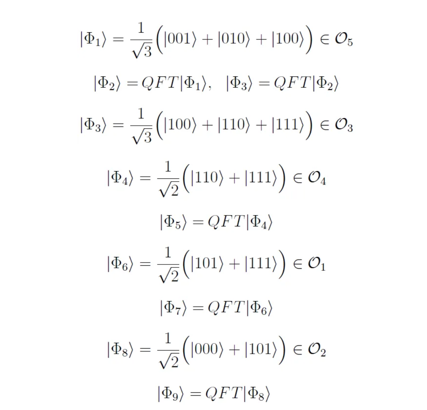
We regroup in the figure below all the possible moves between the defined states and their SLOCC orbits. We observe that, by starting from a given entanglement class, we can reach any other state of any other SLOCC orbit by applying a succession of SLOCC and QFT operations.

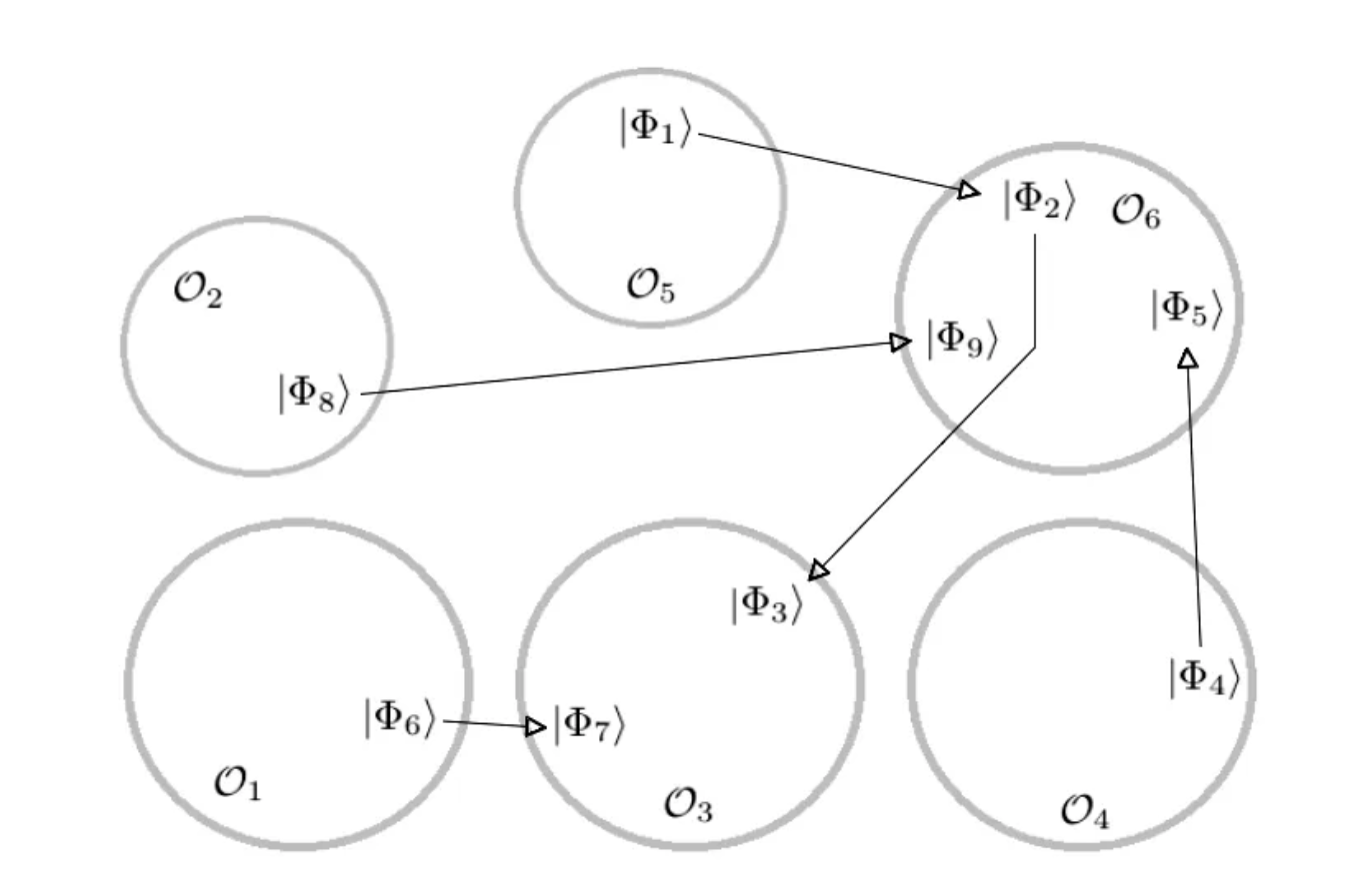
We can then conclude that we only have one unique orbit under the action of the group formed by the union of SLOCC and QFT, in both 2 and 3-qubits cases. This implies that the Quantum Fourier Transform has the ability to modify and create entanglement, and thus can have a huge impact on the speedup of quantum algorithms (as is the case for Shor’s algorithm and Quantum Phase Estimation).

There is hope that this result could be generalized to higher dimensions. However, in the 4-qubit case, the number of SLOCC orbits is already infinite, and dealing with families (for instance [Verstraete2002]) can be a possible solution.

At ColibrITD

At ColibrITD, we believe that understanding deeply the key operations and elements of quantum algorithmic design is essential for developing future quantum algorithms.

Being able to explain the quantum speedup by means of type and amount of entanglement present in the circuit could be a major step in this direction. And the Quantum Fourier Transform is, without doubt, a central operator in Quantum Computing.

Understanding how it acts on a given state and on its fundamental quantum properties (such as entanglement) will help design better quantum algorithms, and will also help leverage the power of quantum computers. In the actual NISQ era, and even in the future, being able to exploit the key resource that is entanglement can help us design in a better and smarter way the quantum circuits (such as Variational Quantum Circuits), in order to minimize their depth and their associated operational error …

And this is exactly what we do at ColibrITD.

References

• [W]: https://en.wikipedia.org/wiki/Fourier_transform
• [W2]: https://en.wikipedia.org/wiki/Discrete_Fourier_transform
[Jaffali2019] : Jaffali, H., Holweck, F. Quantum entanglement involved in Grover’s and Shor’s algorithms: the four-qubit case. Quantum Inf Process 18, 133 (2019)
• [Nielsen2011]: Michael A. Nielsen and Isaac L. Chuang, Quantum computation and quantum information : 10th anniversary edition, 2011.
• [Jaffali2020]: Hamza Jaffali. Étude de l’Intrication dans les Algorithmes Quantiques : Approche Géométrique et Outils Dérivés. Thesis : Université Bourgogne Franche-Comté, (2020)
• [Verstraete2002]: Frank Verstraete, J Dehaene, B De Moor, and Henri Verschelde, Four qubits can be entangled in nine different ways, Physical Review A, 65 (2002), no. 5, 52112.
• [Most2010]: Yonatan Most, Yishai Shimoni, and Ofer Biham, Entanglement of periodic states, the quantum fourier transform, and shor’s factoring algorithm, Physical Review A 81 (2010), no. 5, 52306.